Sample Experimental Results
The results below come from Bachelor student projects carried out at Saarland University within the Systems Engineering programme. They demonstrate the platform’s capacity to support a natural learning progression from classical linear control to nonlinear optimisation-based methods, and from closed-loop control to system identification, all on the same physical hardware.
LQR vs. MPC: Swing-Up and Balancing
Two controllers were implemented and compared on the single-pendulum configuration:
- LQR (Linear Quadratic Regulator): the nonlinear system is linearised around a reference trajectory computed offline. The resulting time-varying linear controller runs directly on the embedded microcontroller at 1 kHz.
- MPC (Model Predictive Control): a nonlinear model is solved online at each time step on a personal computer at 0.1 kHz, providing an optimisation-aware treatment of the full swing-up and balancing task.
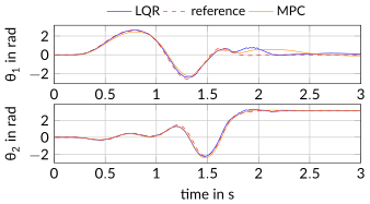
Both controllers successfully swing the pendulum up and stabilise it in the upright position. The comparison highlights a fundamental trade-off in control engineering: the MPC solution is more constrained and optimisation-aware, but demands significantly more computation. This trade-off is itself a core teaching point that students experience directly on real hardware.
We gratefully acknowledge M. Klein, who obtained these results during his project work in our group.
Parameter Identification: From Linear Regression to Nonlinear Collocation
A two-step system identification workflow was applied to measured joint-angle trajectories of the two-pendulum configuration.
In the first step, angular velocities and accelerations are estimated from encoder signals and used to cast the identification problem as a linear regression in the unknown physical parameters (masses, inertias, and link lengths). This yields a fast, closed-form initial estimate.
In the second step, the linear-regression result initialises a nonlinear optimisation that fits the full equations of motion to the measured trajectory using a collocation discretisation, refining the parameter estimates where transient and coupling dynamics are most significant.
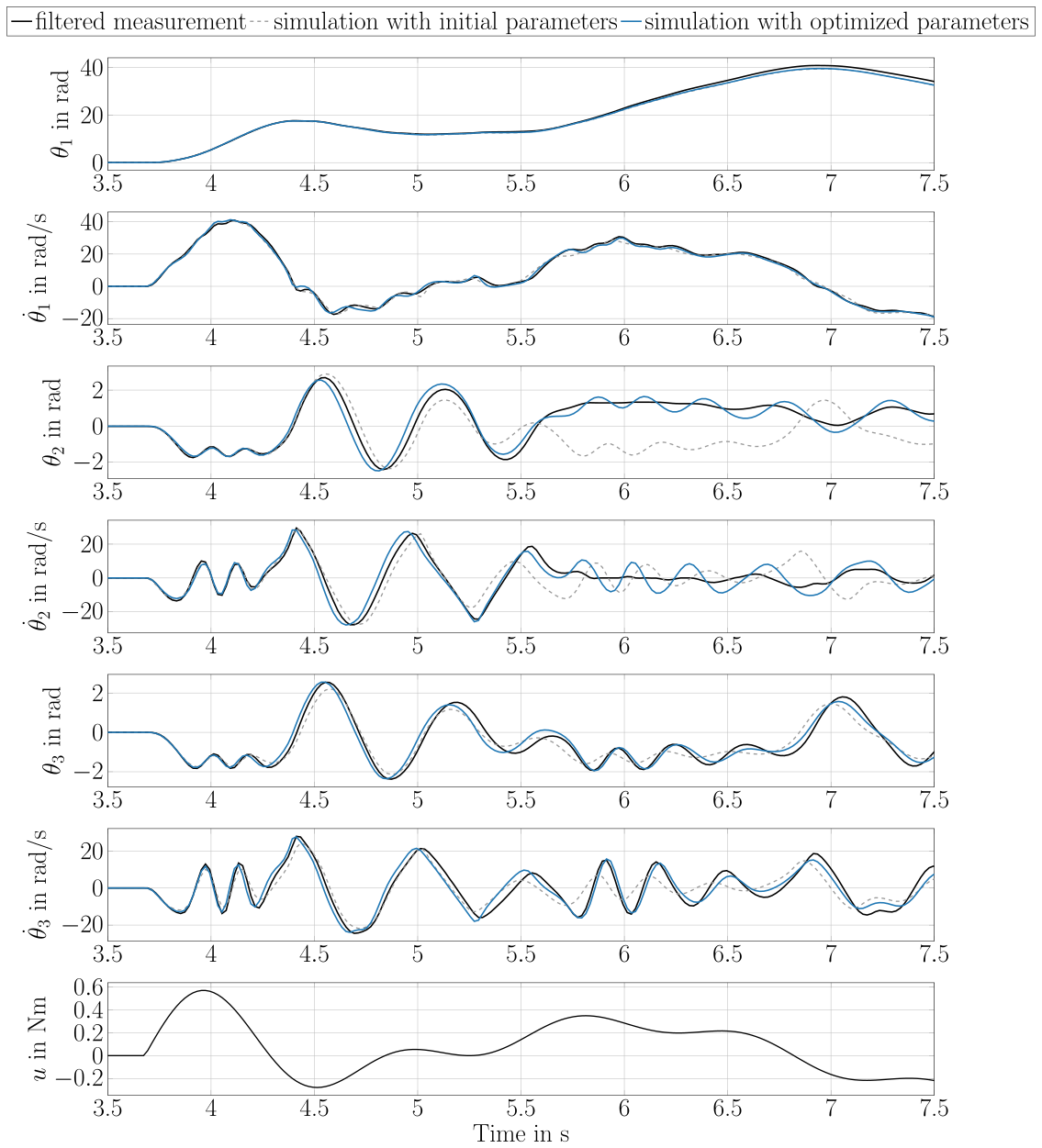
The optimised parameters closely reproduce the measured trajectories across all three joints, including the transient phases where coupling between the two pendulum links is most pronounced. The two-step approach illustrates a practically motivated progression that students can follow from a transparent algebraic method to a rigorous nonlinear optimisation, both grounded in real experimental data.